Operators
The calculator has operators for expressing calculations, such as plus or minus. The full list of operators appears below. They appear essentially in the order of precedence in which they are interpreted in the calculator.
Unit Operators
| u:², u:³ | Unit square, unit cube |
| √:u, ∛:u, ∜:u | Unit square root, unit cube root, unit fourth root |
| u^:n | Unit power |
| u/:u, u per u | Unit divide |
| u*:u, u⋅u, u-:u | Unit multiply |
| n in u | Conversion operator |
Mathematical Operators
| +n, -n | Unary plus, unary minus |
| n' | Transpose |
| n%, n‰, n‱ | Percent, Permille, Basis points |
| n², n³ | Square, cube |
| ∠n | Angle of |
| √n, ∛n, ∜n | Square root, cube root, fourth root |
| n^n, n**n | Matrixwise power |
| n.^n, n.**n | Elementwise power |
| n√n | nth root |
| n*n, n×n, n∗n | Matrixwise times |
| n.*n | Elementwise times |
| n/n, n∕n | Matrixwise divide |
| n./n, n.∕n, n÷n | Elementwise divide |
| n\n | Left divide |
| n%n | Modulus |
| n+n, n-n | Plus, minus |
| n∠n | Angle entry |
| n<<n | Shift left |
| n>>n | Shift right |
| n>>>n | Unsigned shift right |
| n<n | Less than |
| n<=n, n≤n | Less than or equal to |
| n>n | Greater than |
| n>=n, n≥n | Greater than or equal to |
| n==n | Equals |
| n!=n, n~=n, n≠n | Not equals |
| n≈n | Approximately equals |
| n||n, n∥n | Parallel |
| n:n:n | Range (specified step) |
| n:n | Range (step of 1) |
Logical Operators
| !b, ~b | Not |
| b==b, | Equals |
| b!=b, b~=b, b≠b | Not equals |
| b&b, b∧b | And |
| b⊕b | Exclusive or |
| b|b, b∨b | Or |
| b&&b | Shortcut and |
| b||b, b∥b | Shortcut or |
| b?n:n | Choice operator |
String Operator
| s+s | Combine (Concatenate) |
Assignment Operators
| n++, n-- | Increment, decrement |
| ++n, --n | Increment, decrement |
| x^=n | Power assignment |
| x*=n, x×=n, x∗=n | Matrixwise multiply assignment |
| x.*=n | Elementwise multiply assignment |
| x/=n, x∕n | Matrixwise divide multiply assignment |
| x./=n | Elementwise multiply assignment |
| x%=n | Modulus assignment |
| x+=n, x-=n | Plus assignment, Minus assignment |
| x&=b, x∧=n | And assignment |
| x|=b, x∨=n | Or assignment |
| x&&=n | Shortcut and assignment |
| x||=n, x∥=n | Shortcut or assignment |
| x<<=n | Left shift assignment, |
| x>>=n | right shift assignment, |
| x>>>=n | unsigned right shift assignment |
| x=n | Assignment |
Unit Operators
Conversion Operator: in
Units
The in operator can be used to convert a value in one unit to another unit or display the value in another base or form. For example convert a length in metres to feet
If a scale factor is used in the unit to convert to then the value will be displayed using that scale factor even if it is not the optimal scale factor for that value
Note that the in operator only needs to be used to show a value in a particular unit, the calculator automatically manages conversion of units to work consistently when applying mathematical operators
In can only convert between units that are measures of the same thing (specifically have the same dimensions)
The in operator can also be used to attach a unit to dimensionless (without unit) quantities for example if it is generated using a function or other operator
Similarly the unit of any quantity can be removed by using the in operator with unit 'dimensionless' or 'one' on the right hand side
Note that removing units from quantities in this way is not generally recommended because it doesn't usually make physical sense and because it requires making assumptions about exactly which unit the value is in.
Bases
The in operator can also be used to display a result in a base other than that currently chosen as the default in the calculator. For example to display a value in hexadecimal
The supported bases are shown in the following table
| Base | Short form | Long form |
|---|---|---|
| 2 | bin | binary |
| 8 | oct | octal |
| 10 | dec | decimal |
| 16 | hex | hexadecimal |
Several in operators can be chained up for expression in a more specific forms, however only the right most unit in, for example, sets the unit will actually appear
Parts-per Form
The in operator can also be used to display dimensionless quantities in forms such as percent or parts per million
The supported forms appear in the following table
| Parts per | Short form | Long form | |
|---|---|---|---|
| Percent | 100 | %, pc, pct, pct. | percent |
| Permille | 1000 | ‰ | permille, permill, permil |
| Basis points | 10000 | ‱, bp | basis points |
| Parts per million | 1000000 | ppm | |
| Parts per billion | 109 | ppb | |
| Parts per trillion | 1012 | ppt | |
| Parts per quadrillion | 1015 | ppq |
Note that, as with base conversions, parts-per conversions don't change the value itself, they merely change the way that it is displayed.
Display Precision
Usually when doing real world calculations you don't need a very high degree of precision in the result because most physical systems don't operate with such precision. To make it easy to use the results of the calculations ODCalc by default rounds its answers to about 5 decimal places (less are shown if the final digits would be zeros).
Internally ODCalc works to a much higher degree of precision (specifically it uses double precision floating point numbers). If more precision in the result is needed then this can be seen using the 'in full' operator
Other Unit Operators
The other unit operators – unit power, unit multiply, unit divide, unit square, cube, square root, cube root and fourth root – allow complex units to be entered. They also allow the unit of a value to be modified, for example (1m + 1ft) /: second = 1.3048 m/s, however this use is discouraged, (1m + 1ft) / 1 second = 1.3048 m/s makes more physical sense. Further details of these unit operators can be seen in the entering numbers section
Mathematical Operators
ODCalc supports a wide set of mathematical operators, many of which will be familiar from use of a desktop calculator or other programming language. There are a few differences, however, such as the matrixwise vs elementwise operators, parallel operator, range operator, percent operator, etc., which will be covered in more detail in this section.
Adding and Subtracting
Addition and subtraction are performed using the + and - operators
They also act as unary minus (i.e. change sign) and unary plus
If both the arguments are arrays or matrices of the same size then the operation is performed elementwise, that is each element of the result is obtained by applying the operator to the corresponding element of each argument array or matrix
If the arguments were of different sizes in the previous example the calculator would have shown an error message. If one of the arguments is a scalar (singular) value and the other an array or matrix then the result is obtained by applying the operator between each element of the array or matrix and the scalar value
Multiplication and Division
Multiplication and division use the * and / operators, however these come in two forms, matrixwise (* and /) and elementwise (.* and ./). If either argument is a scalar then both forms of the operators work identically
However if both arguments are arrays or matrices then the operators work differently. The elementwise operators apply to the corresponding elements of each array or matrices (both must be the same size)
where as the matrixwise operators perform matrix multiply and matrix solve respectively
Powers
Like multiply and divide, the power operator ^ or ** comes in an elementwise and a matrixwise forms. In both cases the second argument must be a scalar, where as the first can be a scalar or a vector or matrix. The elementwise form applies the power to each element in turn
where as the matrixwise form (will!) perform matrix multiplication on the first arg the number of times specified by the second argument (thus the first argument must be square and the second must be a positive integer).
Operators for specific powers (square ², cube ³, square root √, cube root ∛ and fourth root ∜) all work in an elementwise manner
Parts-per Operators
The percent %, permille‰, and basis points ‱ operators can be used to enter values as, for example, percentages, dividing the value that precedes the operator by 100.
When used on arrays or matrices the operator applied to each element individually
Angle Entry
The angle entry operator ∠ can be used to enter a complex number using its magnitude and argument (angle)
The angle argument should be a number with units of angle, or (less preferred) can be a dimensionless number in which case the assumed angle unit is taken from settings within the calculator.
The magnitude argument can take a unit if desired. It may also be a complex number in which case the complex number is rotated in the complex plane by the given angle
Either or both of the inputs may be complex numbers in which case the operator acts in an elementwise fashion as discussed in the multiplication and division section.
Angle Of
The angle of operator ∠ can be used get the argument (angle) of a complex number
The value returned has dimensions of angle, the unit to be used in specified in settings within the calculator, though of course it can be converted to any other angle unit using the in operator
The input may be an array or matrix in which case the result is an array or matrix with the same size as the input and each element set by applying the angle of operators to the corresponding input element
Parallel
The parallel operator (∥ or two pipe symbols ||) performs the common engineering function of giving the equivalent impedance of two elements in parallel, i.e. applies the following formula
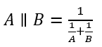
If either of the arguments are arrays or matrices the operator is applied in an elementwise manner as explained the multiplication and division section.
Range
The range operator is useful for creating arrays of values between specified limits, for example between ten and fifteen
The gap between entries can also be specified by using the three argument form, for example between ten and fifteen with a gap of two
Note here that it will fill the range until it encounters a value bigger than the last argument.
The operator is particularly useful for marking off repeated distances during mechanical design, for example two inch divisions between 1.2 and 1.6 metres
or the position of the pins of a 4 way 0.1” gap connector starting at 20mm in an electrical design
The two argument form can also be used with units in which case the gap is the size of unit of the first argument
Comparison Operators
The comparison operators equals (==), not equals (!=, ~= or ≠), approximately equals (≈), less than (<), less than or equal to (<= or ≤), greater than (>) and greater than or equal to (>= or ≥) allow comparison of number values by size, returning logical values as to whether the conditions are true or false.
Units are supported in which case both arguments must have units with the same dimensions
Either or both arguments may be arrays or matrices in which case the operator is applied in an elementwise manner as explained in the multiplication and division section.
If the argument are complex numbers then both the real and imaginary parts of the number must be the same for equals and approximately equals to return true and for not equals to return false
The greater than, less than, greater than or equal to and less than or equal to operators, however, ignore the imaginary part of numbers when making comparisons
The approximately equals operator is included in ODCalc to address machine precision in comparisons. Calculations in computers are performed to within a certain accuracy (they can only keep track of a finite number of digits) meaning that small errors can creep into calculations. For example consider the following sum which results in a number that is very close to but not exactly zero as it should be
The approximately equals operator is tolerant of these small errors when performing comparisons
This is particularly useful when comparing quantities that require conversion between units. (Precisely the approximately equals operator returns true if the quantities are within 100 machine epsilons of each other.)
Logical Operators
Logic operators work on logical values, all returning logical values as a result. When arguments are arrays or matrices the operators are performed elementwise as described in the multiplication and division section.
Not
The not operator, ! or ~ inverts the value
And, Or, Xor
The and operator (& or ∧), or operator (| or ∨) and xor operator (⊕) perform the and, or and xor functions as explained in the following truth table results
Shortcut And and Or
The shortcut and (&&) and or (||) operators work similarly to the standard and and or operators except that they don't evaluate the second argument if the result is already determined by the first argument. For example when evaluating true || false, once the initial true has been found it is not necessary to examine the second argument to determine the result. For constant arguments it makes little difference which form is used (though the shortcut forms as slightly faster)
However these forms are particularly useful when using functions that either modify the state of the system or require the arguments to have certain forms. Note that the shortcut and and or operators only work with scalar arguments.
String Operator
Combine (Concatenate)
The string append operator (+) combines two strings together into a single longer string
If either of the arguments are variables of some type other than string they will first be converted to strings before being appended
For arrays and matrices append works in an elementwise manner
Assignment Operators
The assignment operators store values as variables in the context such as the workspace. In ODCalc variables must be single words without spaces that don't start with a number or an operator character. The must also not begin with the name or symbol of a currency. Once defined they can be used in further calculations until they either go out of scope or are cleared from the workspace.
Equals Assignment
Equals is the most common assignment operator which stores a value in a variable
Unless specified, variables in ODCalc can take any type and be changed to different types even after being declared.